Burr Grinder Particle Size Distribution Analysis

You can analyze a burr grinder’s particle size distribution (PSD) with a DiFluid Omni and a known reference size, then plot the volume‑vs‑diameter curve to see fines (<100 µm) and median particle size. A tight PSD with few fines yields smoother espresso, while excess fines speed extraction and cause bitterness. Larger flat burrs (65 mm+) flatten extremes, reducing boulders and improving uniformity. By normalizing each grinder’s median to a 340 µm reference, you can compare fines propensity and rank performance. Keep exploring to discover how RPM, feed rate, and burr geometry further shape your PSD.

Why Grinder Particle Size Distribution Matters for Espresso

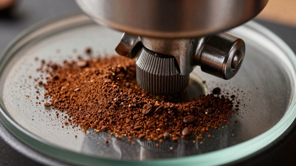
Because espresso extraction hinges on how quickly water contacts coffee, the particle size distribution (PSD) of your grind directly shapes flavor and mouthfeel. You’ll notice that a tight PSD with fewer fines yields a smoother body, while an excess of fines spikes surface area, accelerates brew rate, and can produce bitterness. Burr grinder geometry matters: larger burrs (65 mm+) trim both extreme fines and boulders, tightening the distribution for more even espresso extraction. When you switch settings, the fines fraction shifts, and the presence of oversized particles varies, so each grinder behaves uniquely. Consistent bean roast and a reference median size let you compare how different burrs generate fines, ensuring you target the optimal PSD for balanced espresso. Static reduction can further influence how cleanly grounds disperse into the portafilter, affecting repeatability of the dose.

What Is Grinder Particle Size Distribution and Why It Matters?

You’ve seen how a tight PSD with fewer fines yields a smoother espresso body, but understanding what PSD actually is helps you control that outcome. Particle size distribution (PSD) maps how many coffee fragments fall into each size range, usually plotted on a log‑scale curve of volume versus diameter. The curve shows a nominal peak of coarser particles and a tail of fines—particles under 100 µm that dramatically increase surface area. Burr grinders shape that curve; larger burrs and optimal geometry flatten extremes, producing a more uniform PSD. A well‑balanced PSD steadies extraction dynamics, delivering consistent flavor and avoiding over‑extraction from excessive fines. By grasping these relationships, you can tweak grinder settings, bean load, and calibration to achieve the desired espresso profile. Double-wall vacuum insulation and precise workmanship in mugs for temperature retention highlight how high‑quality construction can influence reliability and performance in daily use.

How to Capture Accurate Grinder Particle Size Distribution Data With Home‑Friendly Tools

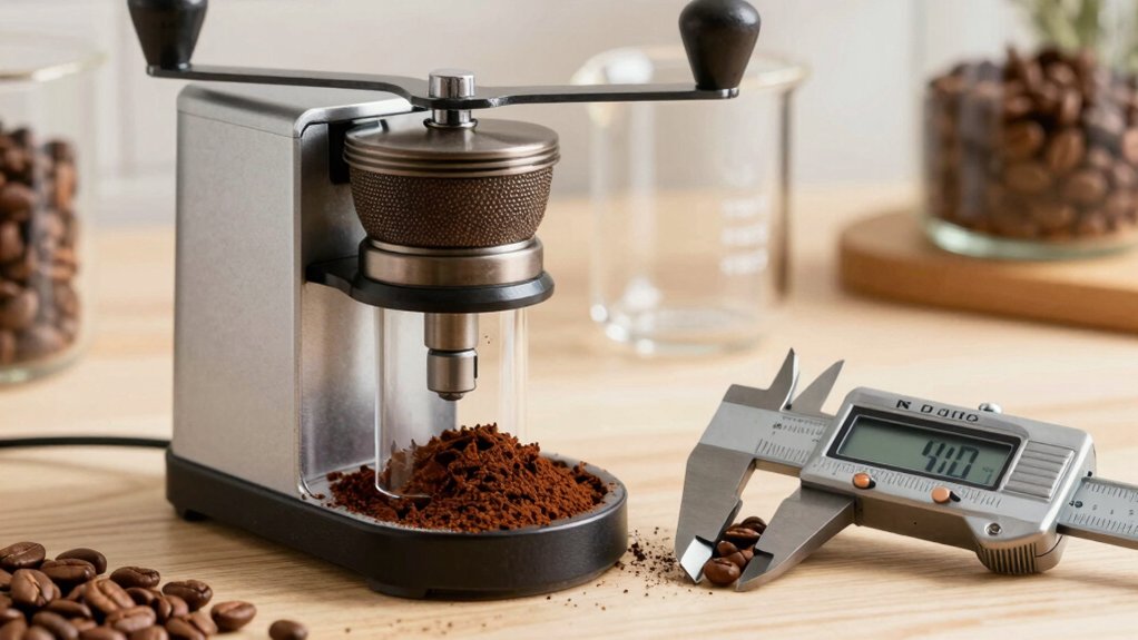
Want to nail down a grinder’s true particle‑size profile without a lab? Grab a DiFluid Omni with CoffeeOS and set up a quick calibration using a known reference size, like 340 µm. Brew five grind settings, each time dispensing a uniform pinch—no more than one‑64th teaspoon—onto a flat surface. Spread the particles, tap gently to break clumps, then run the analyzer to capture the particle size distribution. Record the fines fraction (0–100 µm) and median size for each run, then overlay the curves with MAD shading to see consistency. Normalize results across grinders by referencing the same standard size, and compare results across grinders by normalizing to the same reference, and watch for blade‑grinder chaos that skews the PSD. This routine gives you reliable, home‑friendly data for espresso‑grade burrs. Reference size

Interpreting the Fines Fraction in Grinder Particle Size Distribution

How do you read the fines fraction when you plot it against median particle size? You look at the curve that shows the volume under the particle size distribution from 0 µm to 100 µm as a function of median particle size. A steep rise indicates a grinder that produces many fines at a given grind, while a flat line suggests a more uniform cut. Compare each grinder curve to the 340 µm reference point to normalize across devices; the closer a curve sits to that point, the higher its fines propensity at a common size. Remember that shape matters: a narrow peak of fines can behave differently than a broad distribution, and the presence of boulders will skew extraction despite identical fines fractions. This interpretation guides you in ranking grinders for extraction performance. Grinder Characteristics

Visualizing Fines Across Grinders: Plotting Trends and Median Deviations

After interpreting the fines fraction against median particle size, the next step is to visualize those relationships across multiple grinders. You plot the fines (0–100 µm) as red circles against the median size, overlay a blue polynomial best‑fit, and shade the median absolute deviation region. A vertical green dashed line at 340 µm median size normalizes each grinder’s curve, letting you see how each grinder’s particle size distribution deviates. The trends reveal grinder‑dependent behavior: some grinders spike in fines at finer settings, while others stay flat. This visual framework also extends to boulder analysis, comparing coarse‑particle extents at the same reference point. New insights provide additional context for interpreting the distribution patterns across devices.

Identifying Grind‑Size‑Prone Grinders

Because each grinder’s burr geometry and alignment dictate how fines emerge across the grind range, you can pinpoint which models are truly grind‑size‑prone by comparing their median‑size‑normalized curves. Look for a bell‑shaped fines distribution at coarse settings that collapses into a tight, compressed peak at espresso‑fine levels; that pattern signals a grinder‑specific tendency toward fine‑generation. Larger burrs typically tighten the distribution, suppressing extreme fines and large particles, while smaller burrs broaden it. Use the K6 manual grinder as a benchmark—its shift from a central peak to a slender profile shows how burr geometry drives the curve. By overlaying each grinder’s normalized curve on a common reference (e.g., 340 µm), you isolate the models that consistently produce fines across the grind spectrum. grinder geometry and alignment thus influence the shape of the distribution across settings.

Measuring Boulders and Coarse‑Peak Widths in Grinder Particle Size Distribution

You’ll start by fitting a first‑order polynomial to the PSD at 10 µm and 100 µm, then isolate the right‑hand side of the coarse peak after subtracting a triangle‑shaped curve. This yields two unimodal red distributions whose half‑widths on the right side give you the boulder identification method and the coarse‑peak width metric. Plotting those widths against the median particle diameter lets you see how burr size and geometry affect grinder uniformity. The approach benefits from considering the texture and composition of the grinding materials as described in related analyses Demerara sugar textures and how particle morphology can influence peak broadening in PSD measurements.

Boulder Identification Method

What does a broad right‑side tail in your grinder’s particle‑size distribution (PSD) tell you? It signals boulder presence and hints at grinder uniformity issues. To isolate that signal, you first perform PSD baseline removal, subtracting a triangle‑shaped curve that represents the coarse peak. Then you measure the right‑tail width, comparing it to the median particle diameter and the 340 µm reference line. This process lets you quantify the characteristic half‑width of the boulders, revealing how burr type and grind settings affect the distribution.

1. Fit two unimodal pieces to the baseline‑corrected PSD.
2. Identify the right‑side tail beyond the coarse peak.
3. Calculate the half‑width in microns.
4. Interpret the width as a metric of boulder presence.

Coarse‑Peak Width Metric

The coarse‑peak width metric quantifies how far the right‑side tail of a baseline‑corrected PSD extends beyond the coarse peak, giving you a direct, micron‑scale measure of boulder presence and grinder uniformity. You subtract the triangle‑shaped baseline, then measure the distance from the coarse‑peak apex to the point where the distribution returns to baseline. Larger coarse‑peak width values signal more pronounced boulders, reflecting poorer grinder uniformity and broader particle size distribution.

In boulder analysis you’ll notice the metric shifts with grinder type, grind size, and burr geometry; the Mahlkönig X54, for example, shows a wide right‑side tail that correlates with increased boulder generation. Compare this width against the fines distribution at the 340 µm reference to assess overall performance.

Comparing Flat vs. Conical Grinder Burrs With PSD Metrics

You’ll notice that flat burrs push the fine‑particle fraction higher, while conical burrs keep the overall distribution more uniform.

This contrast shows up clearly in the PSD metrics, where the flat‑burr fines trend spikes and the conical‑burr uniformity metric stays tighter.

Use these differences to gauge how each geometry will affect your espresso extraction consistency.

Flat Burr Fines Trend

Ever notice how flat burrs consistently yield a tighter, monomodal grind while conical burrs scatter particles into a dual‑peak distribution? When you examine the fines trend, flat burrs keep the low‑end tail short, preventing excess powder that can over‑extract. Larger flat burrs (65 mm+) push the fine cutoff upward, so the particle size distribution stays compact and the brew stays balanced. In head‑to‑head tests, the LUCCA Atom’s 75 mm flat burrs produce noticeably fewer fines than the Eureka Mignon Zero’s 55 mm conical burrs, translating to smoother crema and less sludge.

1. Flat burrs → tighter PSD
2. Conical burrs → broader fines spread
3. Larger burrs → reduced extreme fines
4. Consistent fines → predictable extraction

Conical Burr Uniformity Metric

Precision matters when you compare flat and conical burrs, so we introduce a uniformity metric that quantifies how tightly particles cluster around a target size. You calculate it by taking the standard deviation of the particle size distribution (PSD) and dividing it by the mean size, then expressing the result as a percentage. For conical burrs, the metric often reveals a broader spread because their PSD tends to be bi‑modal, especially at smaller grind settings. Larger conical burrs (65 mm+) shrink the tails, pulling the uniformity percentage closer to that of flat burrs, which usually show a narrow, unimodal PSD. Aligning RPM and grind setting to a 340 µm reference lets you compare the two geometries fairly, highlighting how conical burrs affect extraction consistency.

How RPM and Bean Feed Rate Shape Your Grinder PSD Profile

Why does the grind sometimes feel too fine or too coarse even when you keep the setting constant? Your grinder’s RPM and bean feed rate are the hidden levers that reshape the particle size distribution (PSD) and the fines fraction. Faster RPM throws burrs into a more aggressive motion, while a higher bean feed rate pushes more material into the grinding zone, both expanding the PSD tail and often increasing fines. Conversely, slowing RPM or feed can tighten the distribution but may also raise puck resistance, altering extraction. Mastering espresso means balancing these variables, not just tweaking the grind setting.

Grinder RPM and feed rate silently reshape particle size, dictating espresso fine‑coarse perception.

1. Increase RPM → broader PSD, more fines.
2. Decrease RPM → tighter PSD, lower fines.
3. Raise bean feed rate → shift PSD toward finer particles.
4. Lower bean feed rate → coarser PSD, reduced fines.

How to Rank Grinders Using a 340 µm Reference Median

How can you objectively compare grinders when each machine’s settings differ? Start by normalizing every particle size distribution to a 340 µm reference median. Plot the fines fraction against median diameter and draw a vertical green dashed line at 340 µm; this fixed anchor lets you see how far each grinder’s curve deviates. The farther the curve sits above the reference, the higher its propensity for fines formation, regardless of peak height or position. Assign scores based on the vertical distance at the 340 µm point, then rank grinders from lowest to highest fines tendency. This grinder ranking method isolates the effect of grind settings, giving you a clear, comparable metric across all machines.

How to Reduce Fines in Your Grinder Settings

Ever wonder why your espresso sometimes tastes overly sharp or under‑extracted? You can curb those harsh fines by tweaking your grind settings and understanding how burrs shape the particle size distribution. A tighter PSD means fewer sub‑100 µm particles, smoother extraction, and a balanced cup.

Tweak grind settings and burrs to reduce sub‑100 µm fines for smoother, balanced espresso.

1. Use a coarser setting – shift the dial a notch up to cut the volume under the 0‑100 µm range.
2. Check burr alignment – mis‑aligned burrs create irregular cuts that spike fines; clean and reseat them regularly.
3. Choose larger burrs – 65 mm+ burrs generate a more uniform PSD, naturally limiting extreme fines.
4. Adjust bean load – a fuller hopper changes the burr bite, often reducing the fine fraction without sacrificing dose.

These steps let you fine‑tune the grind for a cleaner particle size distribution and a smoother espresso.

Leveraging Large‑Scale PSD Datasets to Choose the Best Grinder for Your Brew

You’ll start by normalizing each grinder’s median particle size to a common reference, then calculate the fine‑particle fraction to see how much waste you’d be pulling through.

Next, compare the boulder generation trends across the dataset to spot models that keep large fragments to a minimum.

Those two metrics together let you pick the grinder that consistently hits your target grind size with the cleanest distribution.

Normalize Median Particle Size

Why compare grinders when their median particle sizes are measured on different scales? You normalize median particle size to a reference size 340 microns, turning disparate PSDs into a common language. This median particle size normalization lets you rank each grinder’s fines fraction at the same point, revealing systematic trends across large datasets. You can then spot grinders that behave similarly or diverge—unimodal versus multimodal distributions—while keeping the particle size distribution comparable.

1. Convert every median to 340 µm using linear interpolation.
2. Plot fines fraction versus the normalized median.
3. Rank grinders by fines at the reference size.
4. Identify consistent trend patterns across devices.

Quantify Fine Particle Fraction

Having normalized each grinder’s median particle size to the 340 µm reference, you can now quantify the fine‑particle fraction that directly impacts extraction and flavor. The fines fraction—volume under the particle size distribution curve from 0 µm to 100 µm—serves as a clear metric for comparing grinders. Large‑scale PSD analysis smooths out noise, letting you see which models consistently produce higher fines at a given median size. Plotting fines fraction against median size reveals unimodal or multimodal trends, helping you rank grinders for consistency and brew quality.

Grinder	Median Size (µm)	Fines Fraction (%)
A	340	12
B	340	8
C	340	15
D	340	9
E	340	11

Use this table to pinpoint the grinder that balances fine particles with overall uniformity.

Evaluate Boulder Generation Trends

How do boulder‑generation trends reveal a grinder’s uniformity across different grind settings? You’ll see that particle size distribution data expose the right‑side width of the coarse peak, measured after subtracting a triangle‑shaped curve. Larger boulder generation widths signal more coarse fragments and lower grinder uniformity. By comparing datasets from Mahlkönig X54 and other units, you can map how burr geometry—conical versus flat—shifts the boulder extent as median particle diameter changes. Polynomial fits illustrate the relationship between grind size, burr gap, and boulder generation, letting you pick the grinder that keeps the coarse tail minimal.

1. Extract right‑side width from PSD.
2. Correlate width with uniformity metrics.
3. Model burr geometry impact.
4. Apply polynomial fits across grind sizes.

Frequently Asked Questions

How Does Bean Roast Level Affect PSD Shape?

You’ll notice darker roasts produce broader, flatter PSDs because the beans become more brittle and shatter, while lighter roasts keep a tighter, peaked distribution, reflecting their firmer structure.

Can Ambient Humidity Alter the Fines Proportion?

Yes, ambient humidity can increase the fines proportion. Moisture makes particles stick together, causing clumping and uneven grinding, which yields more tiny fragments and a broader distribution of fine particles.

Do Different Bean Origins Change Burr Wear Patterns?

Yes, different bean origins affect burr wear. Their varying densities, oil content, and hardness cause distinct abrasion patterns, so you’ll notice faster wear on harder, drier beans and slower wear on softer, oily ones.

What Impact Does Grinder Cleaning Frequency Have on PSD?

You’ll see a cleaner grinder yields a tighter PSD, reducing fines and coarse chunks; frequent cleaning prevents buildup that clogs burrs, so particles stay more uniform and extraction stays consistent.

How Does Static Electricity Influence Particle Clustering During Measurement?

You’ll see static pulling particles together, forming clumps that skew size readings; it attracts opposite charges, causing fine grains to stick, so your distribution appears coarser and less accurate.

In Summary

By now you’ve seen how a grinder’s particle size distribution (PSD) shapes espresso flavor, consistency, and extraction efficiency. Measuring PSD at home, interpreting the fines fraction, and comparing medians against a 340 µm benchmark let you rank grinders objectively. Adjust RPM and feed rate, trim fines, and use large‑scale PSD data to fine‑tune your setup. The result? Consistently better shots, less waste, and a clearer path to your perfect brew.